Fitting TESS data

import exoplanet

exoplanet.utils.docs_setup()
print(f"exoplanet.__version__ = '{exoplanet.__version__}'")

exoplanet.__version__ = '0.5.4.dev27+g75d7fcc'

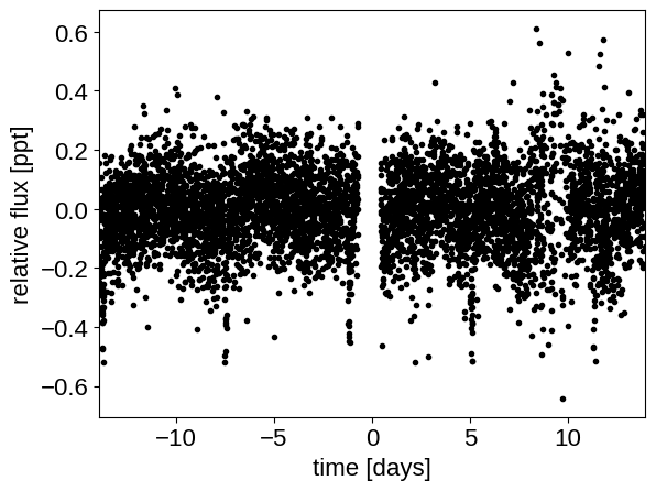
In this tutorial, we will reproduce the fits to the transiting planet in the Pi Mensae system discovered by Huang et al. (2018). The data processing and model are similar to the Joint RV & transit fits case study, but with a few extra bits like aperture selection and de-trending.

To start, we need to download the target pixel file:

import numpy as np
import lightkurve as lk
import matplotlib.pyplot as plt
from astropy.io import fits

lc_file = lk.search_lightcurve(
    "TIC 261136679", sector=1, author="SPOC"
).download(quality_bitmask="hardest", flux_column="pdcsap_flux")
lc = lc_file.remove_nans().normalize().remove_outliers()
time = lc.time.value
flux = lc.flux

# For the purposes of this example, we'll discard some of the data
m = (lc.quality == 0) & (
    np.random.default_rng(261136679).uniform(size=len(time)) < 0.3
)

with fits.open(lc_file.filename) as hdu:
    hdr = hdu[1].header

texp = hdr["FRAMETIM"] * hdr["NUM_FRM"]
texp /= 60.0 * 60.0 * 24.0

ref_time = 0.5 * (np.min(time) + np.max(time))
x = np.ascontiguousarray(time[m] - ref_time, dtype=np.float64)
y = np.ascontiguousarray(1e3 * (flux[m] - 1.0), dtype=np.float64)

plt.plot(x, y, ".k")
plt.xlabel("time [days]")
plt.ylabel("relative flux [ppt]")
_ = plt.xlim(x.min(), x.max())

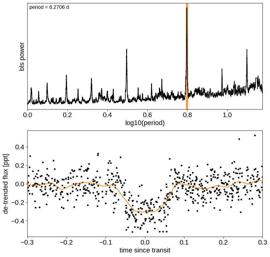
Transit search

Now, let’s use the box least squares periodogram from AstroPy (Note: you’ll need AstroPy v3.1 or more recent to use this feature) to estimate the period, phase, and depth of the transit.

from astropy.timeseries import BoxLeastSquares

period_grid = np.exp(np.linspace(np.log(1), np.log(15), 50000))

bls = BoxLeastSquares(x, y)
bls_power = bls.power(period_grid, 0.1, oversample=20)

# Save the highest peak as the planet candidate
index = np.argmax(bls_power.power)
bls_period = bls_power.period[index]
bls_t0 = bls_power.transit_time[index]
bls_depth = bls_power.depth[index]
transit_mask = bls.transit_mask(x, bls_period, 0.2, bls_t0)

fig, axes = plt.subplots(2, 1, figsize=(10, 10))

# Plot the periodogram
ax = axes[0]
ax.axvline(np.log10(bls_period), color="C1", lw=5, alpha=0.8)
ax.plot(np.log10(bls_power.period), bls_power.power, "k")
ax.annotate(
    "period = {0:.4f} d".format(bls_period),
    (0, 1),
    xycoords="axes fraction",
    xytext=(5, -5),
    textcoords="offset points",
    va="top",
    ha="left",
    fontsize=12,
)
ax.set_ylabel("bls power")
ax.set_yticks([])
ax.set_xlim(np.log10(period_grid.min()), np.log10(period_grid.max()))
ax.set_xlabel("log10(period)")

# Plot the folded transit
ax = axes[1]
x_fold = (x - bls_t0 + 0.5 * bls_period) % bls_period - 0.5 * bls_period
m = np.abs(x_fold) < 0.4
ax.plot(x_fold[m], y[m], ".k")

# Overplot the phase binned light curve
bins = np.linspace(-0.41, 0.41, 32)
denom, _ = np.histogram(x_fold, bins)
num, _ = np.histogram(x_fold, bins, weights=y)
denom[num == 0] = 1.0
ax.plot(0.5 * (bins[1:] + bins[:-1]), num / denom, color="C1")

ax.set_xlim(-0.3, 0.3)
ax.set_ylabel("de-trended flux [ppt]")
_ = ax.set_xlabel("time since transit")

The transit model in PyMC3

The transit model, initialization, and sampling are all nearly the same as the one in Joint RV & transit fits.

import exoplanet as xo
import pymc3 as pm
import aesara_theano_fallback.tensor as tt

import pymc3_ext as pmx
from celerite2.theano import terms, GaussianProcess

phase_lc = np.linspace(-0.3, 0.3, 100)


def build_model(mask=None, start=None):
    if mask is None:
        mask = np.ones(len(x), dtype=bool)
    with pm.Model() as model:
        # Parameters for the stellar properties
        mean = pm.Normal("mean", mu=0.0, sd=10.0)
        u_star = xo.QuadLimbDark("u_star")
        star = xo.LimbDarkLightCurve(u_star)

        # Stellar parameters from Huang et al (2018)
        M_star_huang = 1.094, 0.039
        R_star_huang = 1.10, 0.023
        BoundedNormal = pm.Bound(pm.Normal, lower=0, upper=3)
        m_star = BoundedNormal(
            "m_star", mu=M_star_huang[0], sd=M_star_huang[1]
        )
        r_star = BoundedNormal(
            "r_star", mu=R_star_huang[0], sd=R_star_huang[1]
        )

        # Orbital parameters for the planets
        t0 = pm.Normal("t0", mu=bls_t0, sd=1)
        log_period = pm.Normal("log_period", mu=np.log(bls_period), sd=1)
        period = pm.Deterministic("period", tt.exp(log_period))

        # Fit in terms of transit depth (assuming b<1)
        b = pm.Uniform("b", lower=0, upper=1)
        log_depth = pm.Normal("log_depth", mu=np.log(bls_depth), sigma=2.0)
        ror = pm.Deterministic(
            "ror",
            star.get_ror_from_approx_transit_depth(
                1e-3 * tt.exp(log_depth), b
            ),
        )
        r_pl = pm.Deterministic("r_pl", ror * r_star)

        #         log_r_pl = pm.Normal(
        #             "log_r_pl",
        #             sd=1.0,
        #             mu=0.5 * np.log(1e-3 * np.array(bls_depth))
        #             + np.log(R_star_huang[0]),
        #         )
        #         r_pl = pm.Deterministic("r_pl", tt.exp(log_r_pl))
        #         ror = pm.Deterministic("ror", r_pl / r_star)
        #         b = xo.distributions.ImpactParameter("b", ror=ror)

        ecs = pmx.UnitDisk("ecs", testval=np.array([0.01, 0.0]))
        ecc = pm.Deterministic("ecc", tt.sum(ecs**2))
        omega = pm.Deterministic("omega", tt.arctan2(ecs[1], ecs[0]))
        xo.eccentricity.kipping13("ecc_prior", fixed=True, observed=ecc)

        # Transit jitter & GP parameters
        log_sigma_lc = pm.Normal(
            "log_sigma_lc", mu=np.log(np.std(y[mask])), sd=10
        )
        log_rho_gp = pm.Normal("log_rho_gp", mu=0, sd=10)
        log_sigma_gp = pm.Normal(
            "log_sigma_gp", mu=np.log(np.std(y[mask])), sd=10
        )

        # Orbit model
        orbit = xo.orbits.KeplerianOrbit(
            r_star=r_star,
            m_star=m_star,
            period=period,
            t0=t0,
            b=b,
            ecc=ecc,
            omega=omega,
        )

        # Compute the model light curve
        light_curves = (
            star.get_light_curve(orbit=orbit, r=r_pl, t=x[mask], texp=texp)
            * 1e3
        )
        light_curve = tt.sum(light_curves, axis=-1) + mean
        resid = y[mask] - light_curve

        # GP model for the light curve
        kernel = terms.SHOTerm(
            sigma=tt.exp(log_sigma_gp),
            rho=tt.exp(log_rho_gp),
            Q=1 / np.sqrt(2),
        )
        gp = GaussianProcess(kernel, t=x[mask], yerr=tt.exp(log_sigma_lc))
        gp.marginal("gp", observed=resid)
        #         pm.Deterministic("gp_pred", gp.predict(resid))

        # Compute and save the phased light curve models
        pm.Deterministic(
            "lc_pred",
            1e3
            * star.get_light_curve(
                orbit=orbit, r=r_pl, t=t0 + phase_lc, texp=texp
            )[..., 0],
        )

        # Fit for the maximum a posteriori parameters, I've found that I can get
        # a better solution by trying different combinations of parameters in turn
        if start is None:
            start = model.test_point
        map_soln = pmx.optimize(
            start=start, vars=[log_sigma_lc, log_sigma_gp, log_rho_gp]
        )
        map_soln = pmx.optimize(start=map_soln, vars=[log_depth])
        map_soln = pmx.optimize(start=map_soln, vars=[b])
        map_soln = pmx.optimize(start=map_soln, vars=[log_period, t0])
        map_soln = pmx.optimize(start=map_soln, vars=[u_star])
        map_soln = pmx.optimize(start=map_soln, vars=[log_depth])
        map_soln = pmx.optimize(start=map_soln, vars=[b])
        map_soln = pmx.optimize(start=map_soln, vars=[ecs])
        map_soln = pmx.optimize(start=map_soln, vars=[mean])
        map_soln = pmx.optimize(
            start=map_soln, vars=[log_sigma_lc, log_sigma_gp, log_rho_gp]
        )
        map_soln = pmx.optimize(start=map_soln)

        extras = dict(
            zip(
                ["light_curves", "gp_pred"],
                pmx.eval_in_model([light_curves, gp.predict(resid)], map_soln),
            )
        )

    return model, map_soln, extras


model0, map_soln0, extras0 = build_model()

optimizing logp for variables: [log_rho_gp, log_sigma_gp, log_sigma_lc]

100.00% [51/51 00:00<00:00 logp = 3.460e+03]

message: Optimization terminated successfully.
logp: 3338.1817955372735 -> 3460.3983411347185

optimizing logp for variables: [log_depth]

100.00% [8/8 00:00<00:00 logp = 3.466e+03]

message: Optimization terminated successfully.
logp: 3460.3983411347185 -> 3465.961744172654

optimizing logp for variables: [b]

100.00% [11/11 00:00<00:00 logp = 3.501e+03]

message: Optimization terminated successfully.
logp: 3465.961744172654 -> 3501.4417887424743

optimizing logp for variables: [t0, log_period]

100.00% [20/20 00:00<00:00 logp = 3.507e+03]

message: Optimization terminated successfully.
logp: 3501.4417887424734 -> 3507.3259047021374

optimizing logp for variables: [u_star]

100.00% [10/10 00:00<00:00 logp = 3.511e+03]

message: Optimization terminated successfully.
logp: 3507.3259047021384 -> 3510.723293097444

optimizing logp for variables: [log_depth]

100.00% [8/8 00:00<00:00 logp = 3.514e+03]

message: Optimization terminated successfully.
logp: 3510.723293097444 -> 3514.13173448383

optimizing logp for variables: [b]

100.00% [10/10 00:00<00:00 logp = 3.515e+03]

message: Optimization terminated successfully.
logp: 3514.13173448383 -> 3515.137731047359

optimizing logp for variables: [ecs]

100.00% [17/17 00:00<00:00 logp = 3.516e+03]

message: Optimization terminated successfully.
logp: 3515.137731047359 -> 3515.6567965741333

optimizing logp for variables: [mean]

100.00% [4/4 00:00<00:00 logp = 3.516e+03]

message: Optimization terminated successfully.
logp: 3515.6567965741333 -> 3515.6766245050853

optimizing logp for variables: [log_rho_gp, log_sigma_gp, log_sigma_lc]

100.00% [42/42 00:00<00:00 logp = 3.516e+03]

message: Desired error not necessarily achieved due to precision loss.
logp: 3515.6766245050853 -> 3516.2740955297063

optimizing logp for variables: [log_sigma_gp, log_rho_gp, log_sigma_lc, ecs, log_depth, b, log_period, t0, r_star, m_star, u_star, mean]

100.00% [241/241 00:00<00:00 logp = 3.723e+03]

message: Desired error not necessarily achieved due to precision loss.
logp: 3516.274095529706 -> 3722.5360762943724

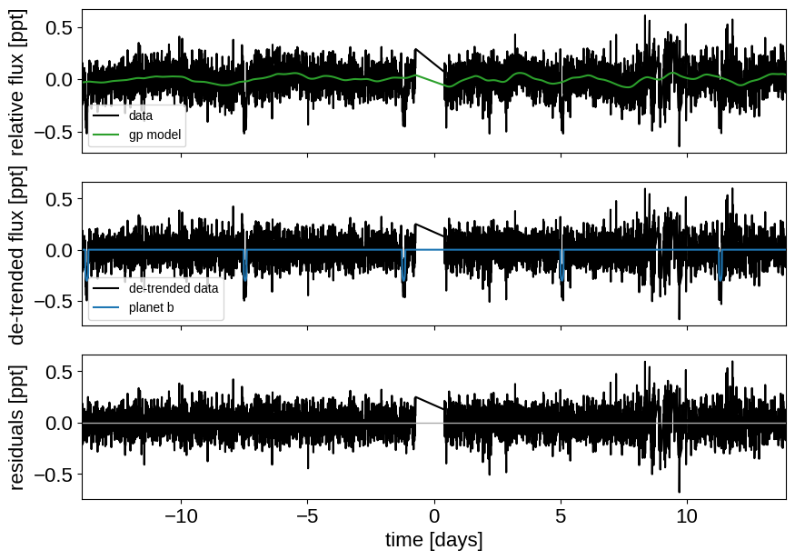
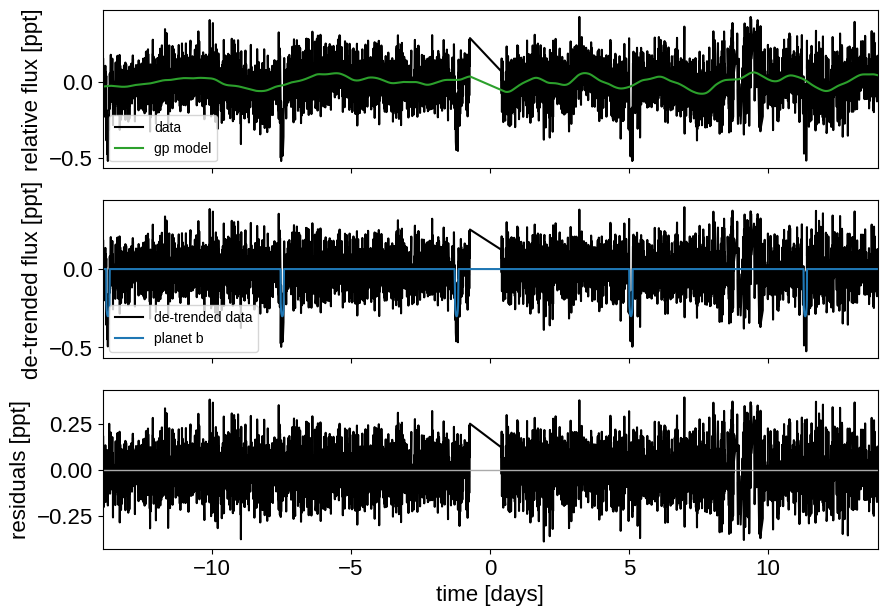
Here’s how we plot the initial light curve model:

def plot_light_curve(soln, extras, mask=None):
    if mask is None:
        mask = np.ones(len(x), dtype=bool)

    fig, axes = plt.subplots(3, 1, figsize=(10, 7), sharex=True)

    ax = axes[0]
    ax.plot(x[mask], y[mask], "k", label="data")
    gp_mod = extras["gp_pred"] + soln["mean"]
    ax.plot(x[mask], gp_mod, color="C2", label="gp model")
    ax.legend(fontsize=10)
    ax.set_ylabel("relative flux [ppt]")

    ax = axes[1]
    ax.plot(x[mask], y[mask] - gp_mod, "k", label="de-trended data")
    for i, l in enumerate("b"):
        mod = extras["light_curves"][:, i]
        ax.plot(x[mask], mod, label="planet {0}".format(l))
    ax.legend(fontsize=10, loc=3)
    ax.set_ylabel("de-trended flux [ppt]")

    ax = axes[2]
    mod = gp_mod + np.sum(extras["light_curves"], axis=-1)
    ax.plot(x[mask], y[mask] - mod, "k")
    ax.axhline(0, color="#aaaaaa", lw=1)
    ax.set_ylabel("residuals [ppt]")
    ax.set_xlim(x[mask].min(), x[mask].max())
    ax.set_xlabel("time [days]")

    return fig


_ = plot_light_curve(map_soln0, extras0)

As in Joint RV & transit fits, we can do some sigma clipping to remove significant outliers.

mod = (
    extras0["gp_pred"]
    + map_soln0["mean"]
    + np.sum(extras0["light_curves"], axis=-1)
)
resid = y - mod
rms = np.sqrt(np.median(resid**2))
mask = np.abs(resid) < 5 * rms

plt.figure(figsize=(10, 5))
plt.plot(x, resid, "k", label="data")
plt.plot(x[~mask], resid[~mask], "xr", label="outliers")
plt.axhline(0, color="#aaaaaa", lw=1)
plt.ylabel("residuals [ppt]")
plt.xlabel("time [days]")
plt.legend(fontsize=12, loc=3)
_ = plt.xlim(x.min(), x.max())

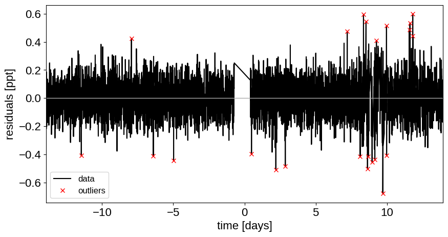
And then we re-build the model using the data without outliers.

model, map_soln, extras = build_model(mask, map_soln0)
_ = plot_light_curve(map_soln, extras, mask)

optimizing logp for variables: [log_rho_gp, log_sigma_gp, log_sigma_lc]

100.00% [15/15 00:00<00:00 logp = 3.886e+03]

message: Optimization terminated successfully.
logp: 3880.262483379479 -> 3886.439828473729

optimizing logp for variables: [log_depth]

100.00% [6/6 00:00<00:00 logp = 3.886e+03]

message: Optimization terminated successfully.
logp: 3886.439828473729 -> 3886.4414819670956

optimizing logp for variables: [b]

100.00% [7/7 00:00<00:00 logp = 3.886e+03]

message: Optimization terminated successfully.
logp: 3886.4414819670956 -> 3886.441650516504

optimizing logp for variables: [t0, log_period]

100.00% [40/40 00:00<00:00 logp = 3.886e+03]

message: Desired error not necessarily achieved due to precision loss.
logp: 3886.4416505165045 -> 3886.4418199582783

optimizing logp for variables: [u_star]

100.00% [6/6 00:00<00:00 logp = 3.886e+03]

message: Optimization terminated successfully.
logp: 3886.441819958278 -> 3886.441904696529

optimizing logp for variables: [log_depth]

100.00% [5/5 00:00<00:00 logp = 3.886e+03]

message: Optimization terminated successfully.
logp: 3886.441904696529 -> 3886.441910233041

optimizing logp for variables: [b]

100.00% [6/6 00:00<00:00 logp = 3.886e+03]

message: Optimization terminated successfully.
logp: 3886.441910233041 -> 3886.4419208006507

optimizing logp for variables: [ecs]

100.00% [7/7 00:00<00:00 logp = 3.886e+03]

message: Optimization terminated successfully.
logp: 3886.44192080065 -> 3886.4419209254083

optimizing logp for variables: [mean]

100.00% [4/4 00:00<00:00 logp = 3.886e+03]

message: Optimization terminated successfully.
logp: 3886.4419209254097 -> 3886.444210713328

optimizing logp for variables: [log_rho_gp, log_sigma_gp, log_sigma_lc]

100.00% [9/9 00:00<00:00 logp = 3.886e+03]

message: Optimization terminated successfully.
logp: 3886.444210713328 -> 3886.444220152795

optimizing logp for variables: [log_sigma_gp, log_rho_gp, log_sigma_lc, ecs, log_depth, b, log_period, t0, r_star, m_star, u_star, mean]

100.00% [104/104 00:00<00:00 logp = 3.886e+03]

message: Desired error not necessarily achieved due to precision loss.
logp: 3886.444220152795 -> 3886.4442436117993

Now that we have the model, we can sample:

import platform

with model:
    trace = pm.sample(
        tune=1500,
        draws=1000,
        start=map_soln,
        # Parallel sampling runs poorly or crashes on macos
        cores=1 if platform.system() == "Darwin" else 2,
        chains=2,
        target_accept=0.95,
        return_inferencedata=True,
        random_seed=[261136679, 261136680],
        init="adapt_full",
    )

Auto-assigning NUTS sampler...

Initializing NUTS using adapt_full...

Multiprocess sampling (2 chains in 2 jobs)

NUTS: [log_sigma_gp, log_rho_gp, log_sigma_lc, ecs, log_depth, b, log_period, t0, r_star, m_star, u_star, mean]

100.00% [5000/5000 08:31<00:00 Sampling 2 chains, 0 divergences]

Sampling 2 chains for 1_500 tune and 1_000 draw iterations (3_000 + 2_000 draws total) took 513 seconds.

import arviz as az

az.summary(
    trace,
    var_names=[
        "omega",
        "ecc",
        "r_pl",
        "b",
        "t0",
        "period",
        "r_star",
        "m_star",
        "u_star",
        "mean",
    ],
)

	mean	sd	hdi_3%	hdi_97%	mcse_mean	mcse_sd	ess_bulk	ess_tail	r_hat
omega	0.450	1.785	-2.817	3.129	0.056	0.040	1139.0	1690.0	1.0
ecc	0.221	0.147	0.000	0.485	0.006	0.005	720.0	758.0	1.0
r_pl	0.018	0.001	0.017	0.020	0.000	0.000	1196.0	1384.0	1.0
b	0.455	0.222	0.028	0.773	0.009	0.007	573.0	630.0	1.0
t0	-13.734	0.002	-13.739	-13.731	0.000	0.000	1333.0	1412.0	1.0
period	6.269	0.001	6.267	6.270	0.000	0.000	1703.0	1527.0	1.0
r_star	1.100	0.023	1.057	1.143	0.001	0.000	1927.0	1367.0	1.0
m_star	1.097	0.038	1.024	1.167	0.001	0.001	1826.0	1486.0	1.0
u_star[0]	0.302	0.227	0.000	0.704	0.006	0.004	1466.0	1054.0	1.0
u_star[1]	0.219	0.307	-0.304	0.807	0.008	0.006	1319.0	1162.0	1.0
mean	0.002	0.007	-0.012	0.016	0.000	0.000	1699.0	1098.0	1.0

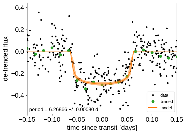
Results

After sampling, we can make the usual plots. First, let’s look at the folded light curve plot:

flat_samps = trace.posterior.stack(sample=("chain", "draw"))

# Compute the GP prediction
gp_mod = extras["gp_pred"] + map_soln["mean"]  # np.median(
#     flat_samps["gp_pred"].values + flat_samps["mean"].values[None, :], axis=-1
# )

# Get the posterior median orbital parameters
p = np.median(flat_samps["period"])
t0 = np.median(flat_samps["t0"])

# Plot the folded data
x_fold = (x[mask] - t0 + 0.5 * p) % p - 0.5 * p
plt.plot(x_fold, y[mask] - gp_mod, ".k", label="data", zorder=-1000)

# Overplot the phase binned light curve
bins = np.linspace(-0.41, 0.41, 50)
denom, _ = np.histogram(x_fold, bins)
num, _ = np.histogram(x_fold, bins, weights=y[mask])
denom[num == 0] = 1.0
plt.plot(
    0.5 * (bins[1:] + bins[:-1]), num / denom, "o", color="C2", label="binned"
)

# Plot the folded model
pred = np.percentile(flat_samps["lc_pred"], [16, 50, 84], axis=-1)
plt.plot(phase_lc, pred[1], color="C1", label="model")
art = plt.fill_between(
    phase_lc, pred[0], pred[2], color="C1", alpha=0.5, zorder=1000
)
art.set_edgecolor("none")

# Annotate the plot with the planet's period
txt = "period = {0:.5f} +/- {1:.5f} d".format(
    np.mean(flat_samps["period"].values), np.std(flat_samps["period"].values)
)
plt.annotate(
    txt,
    (0, 0),
    xycoords="axes fraction",
    xytext=(5, 5),
    textcoords="offset points",
    ha="left",
    va="bottom",
    fontsize=12,
)

plt.legend(fontsize=10, loc=4)
plt.xlim(-0.5 * p, 0.5 * p)
plt.xlabel("time since transit [days]")
plt.ylabel("de-trended flux")
_ = plt.xlim(-0.15, 0.15)

And a corner plot of some of the key parameters:

import corner
import astropy.units as u

trace.posterior["r_earth"] = (
    trace.posterior["r_pl"].coords,
    (trace.posterior["r_pl"].values * u.R_sun).to(u.R_earth).value,
)

_ = corner.corner(
    trace,
    var_names=["period", "r_earth", "b", "ecc"],
    labels=[
        "period [days]",
        "radius [Earth radii]",
        "impact param",
        "eccentricity",
    ],
)

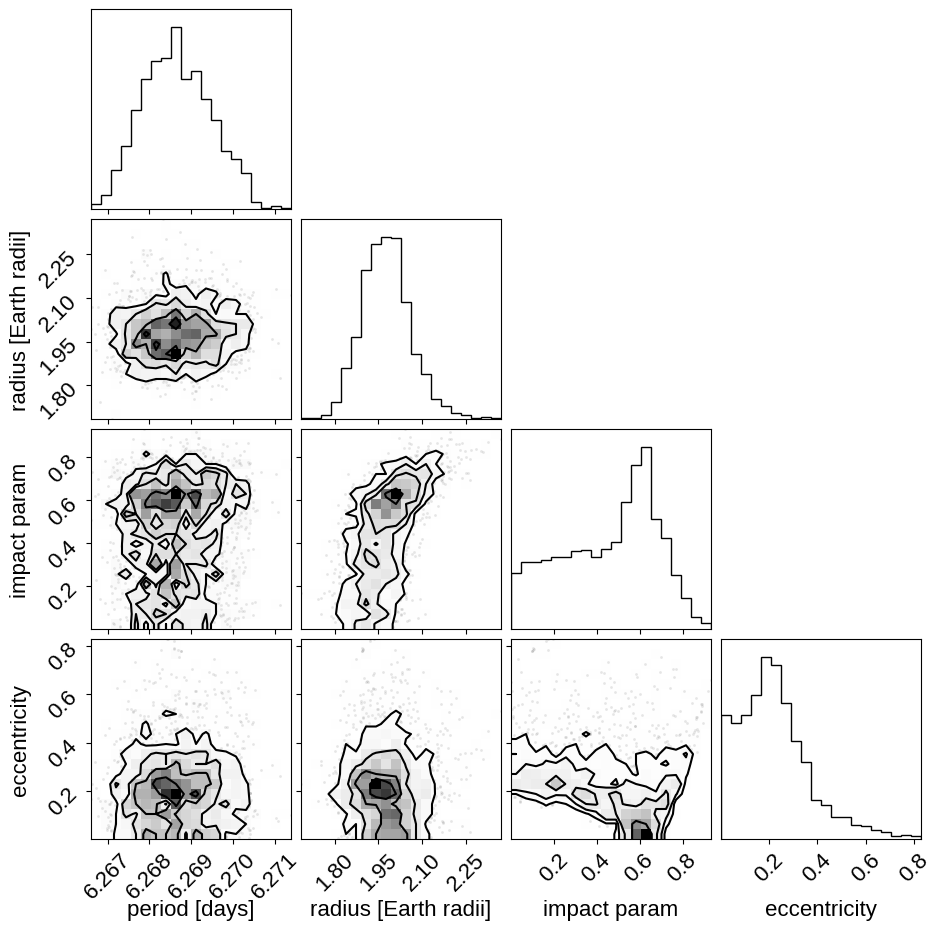
These all seem consistent with the previously published values.

Citations

As described in the citation tutorial, we can use citations.get_citations_for_model to construct an acknowledgement and BibTeX listing that includes the relevant citations for this model.

with model:
    txt, bib = xo.citations.get_citations_for_model()
print(txt)

This research made use of \textsf{exoplanet} \citep{exoplanet:joss,
exoplanet:zenodo} and its dependencies \citep{celerite2:foremanmackey17,
celerite2:foremanmackey18, exoplanet:agol20, exoplanet:arviz,
exoplanet:astropy13, exoplanet:astropy18, exoplanet:kipping13,
exoplanet:kipping13b, exoplanet:luger18, exoplanet:pymc3, exoplanet:theano}.

print(bib.split("\n\n")[0] + "\n\n...")

@article{exoplanet:joss,
       author = {{Foreman-Mackey}, Daniel and {Luger}, Rodrigo and {Agol}, Eric
                and {Barclay}, Thomas and {Bouma}, Luke G. and {Brandt},
                Timothy D. and {Czekala}, Ian and {David}, Trevor J. and
                {Dong}, Jiayin and {Gilbert}, Emily A. and {Gordon}, Tyler A.
                and {Hedges}, Christina and {Hey}, Daniel R. and {Morris},
                Brett M. and {Price-Whelan}, Adrian M. and {Savel}, Arjun B.},
        title = "{exoplanet: Gradient-based probabilistic inference for
                  exoplanet data \& other astronomical time series}",
      journal = {arXiv e-prints},
         year = 2021,
        month = may,
          eid = {arXiv:2105.01994},
        pages = {arXiv:2105.01994},
archivePrefix = {arXiv},
       eprint = {2105.01994},
 primaryClass = {astro-ph.IM},
       adsurl = {https://ui.adsabs.harvard.edu/abs/2021arXiv210501994F},
      adsnote = {Provided by the SAO/NASA Astrophysics Data System}
}

...