Gaussian process models for stellar variability#
import exoplanet

exoplanet.utils.docs_setup()
print(f"exoplanet.__version__ = '{exoplanet.__version__}'")
exoplanet.__version__ = '0.5.4.dev27+g75d7fcc'
When fitting exoplanets, we also need to fit for the stellar variability and Gaussian Processes (GPs) are often a good descriptive model for this variation. PyMC3 has support for all sorts of general GP models, but exoplanet interfaces with the celerite2 library to provide support for scalable 1D GPs (take a look at the Getting started tutorial on the celerite2 docs for a crash course) that can work with large datasets. In this tutorial, we go through the process of modeling the light curve of a rotating star observed by Kepler using exoplanet and celerite2.
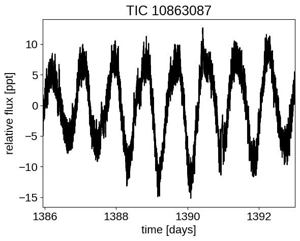
First, let’s download and plot the data:
import numpy as np
import lightkurve as lk
import matplotlib.pyplot as plt

lcf = lk.search_lightcurve(
    "TIC 10863087", mission="TESS", author="SPOC"
).download_all(quality_bitmask="hardest", flux_column="pdcsap_flux")
lc = lcf.stitch().remove_nans().remove_outliers()
lc = lc[:5000]
_, mask = lc.flatten().remove_outliers(sigma=3.0, return_mask=True)
lc = lc[~mask]

x = np.ascontiguousarray(lc.time.value, dtype=np.float64)
y = np.ascontiguousarray(lc.flux, dtype=np.float64)
yerr = np.ascontiguousarray(lc.flux_err, dtype=np.float64)
mu = np.mean(y)
y = (y / mu - 1) * 1e3
yerr = yerr * 1e3 / mu

plt.plot(x, y, "k")
plt.xlim(x.min(), x.max())
plt.xlabel("time [days]")
plt.ylabel("relative flux [ppt]")
_ = plt.title("TIC 10863087")
Warning: 33% (6455/19412) of the cadences will be ignored due to the quality mask (quality_bitmask=8191).
A Gaussian process model for stellar variability#
This looks like the light curve of a rotating star, and it has been shown that it is possible to model this variability by using a quasiperiodic Gaussian process. To start with, let’s get an estimate of the rotation period using the Lomb-Scargle periodogram:
import exoplanet as xo

results = xo.estimators.lomb_scargle_estimator(
    x, y, max_peaks=1, min_period=0.1, max_period=2.0, samples_per_peak=50
)

peak = results["peaks"][0]
freq, power = results["periodogram"]
plt.plot(1 / freq, power, "k")
plt.axvline(peak["period"], color="k", lw=4, alpha=0.3)
plt.xlim((1 / freq).min(), (1 / freq).max())
plt.yticks([])
plt.xlabel("period [days]")
_ = plt.ylabel("power")
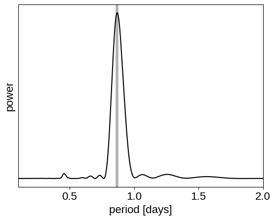
Now, using this initialization, we can set up the GP model in exoplanet and celerite2. We’ll use the RotationTerm kernel that is a mixture of two simple harmonic oscillators with periods separated by a factor of two. As you can see from the periodogram above, this might be a good model for this light curve and I’ve found that it works well in many cases.
import pymc3 as pm
import pymc3_ext as pmx
import aesara_theano_fallback.tensor as tt
from celerite2.theano import terms, GaussianProcess

with pm.Model() as model:
    # The mean flux of the time series
    mean = pm.Normal("mean", mu=0.0, sigma=10.0)

    # A jitter term describing excess white noise
    log_jitter = pm.Normal("log_jitter", mu=np.log(np.mean(yerr)), sigma=2.0)

    # A term to describe the non-periodic variability
    sigma = pm.InverseGamma(
        "sigma", **pmx.estimate_inverse_gamma_parameters(1.0, 5.0)
    )
    rho = pm.InverseGamma(
        "rho", **pmx.estimate_inverse_gamma_parameters(0.5, 2.0)
    )

    # The parameters of the RotationTerm kernel
    sigma_rot = pm.InverseGamma(
        "sigma_rot", **pmx.estimate_inverse_gamma_parameters(1.0, 5.0)
    )
    log_period = pm.Normal("log_period", mu=np.log(peak["period"]), sigma=2.0)
    period = pm.Deterministic("period", tt.exp(log_period))
    log_Q0 = pm.HalfNormal("log_Q0", sigma=2.0)
    log_dQ = pm.Normal("log_dQ", mu=0.0, sigma=2.0)
    f = pm.Uniform("f", lower=0.1, upper=1.0)

    # Set up the Gaussian Process model
    kernel = terms.SHOTerm(sigma=sigma, rho=rho, Q=1 / 3.0)
    kernel += terms.RotationTerm(
        sigma=sigma_rot,
        period=period,
        Q0=tt.exp(log_Q0),
        dQ=tt.exp(log_dQ),
        f=f,
    )
    gp = GaussianProcess(
        kernel,
        t=x,
        diag=yerr**2 + tt.exp(2 * log_jitter),
        mean=mean,
        quiet=True,
    )

    # Compute the Gaussian Process likelihood and add it into the
    # the PyMC3 model as a "potential"
    gp.marginal("gp", observed=y)

    # Compute the mean model prediction for plotting purposes
    pm.Deterministic("pred", gp.predict(y))

    # Optimize to find the maximum a posteriori parameters
    map_soln = pmx.optimize()
optimizing logp for variables: [f, log_dQ, log_Q0, log_period, sigma_rot, rho, sigma, log_jitter, mean]
message: Desired error not necessarily achieved due to precision loss.
logp: -9263.87083670822 -> -8861.082439762553
Now that we have the model set up, let’s plot the maximum a posteriori model prediction.
plt.plot(x, y, "k", label="data")
plt.plot(x, map_soln["pred"], color="C1", label="model")
plt.xlim(x.min(), x.max())
plt.legend(fontsize=10)
plt.xlabel("time [days]")
plt.ylabel("relative flux [ppt]")
_ = plt.title("TIC 10863087; map model")
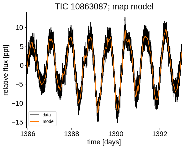
That looks pretty good! Now let’s sample from the posterior using the PyMC3 Extras (pymc3-ext) library:
with model:
    trace = pmx.sample(
        tune=1000,
        draws=1000,
        start=map_soln,
        cores=2,
        chains=2,
        target_accept=0.9,
        return_inferencedata=True,
        random_seed=[10863087, 10863088],
    )
Multiprocess sampling (2 chains in 2 jobs)
NUTS: [f, log_dQ, log_Q0, log_period, sigma_rot, rho, sigma, log_jitter, mean]
Sampling 2 chains for 1_000 tune and 1_000 draw iterations (2_000 + 2_000 draws total) took 131 seconds.
Now we can do the usual convergence checks:
import arviz as az

az.summary(
    trace,
    var_names=[
        "f",
        "log_dQ",
        "log_Q0",
        "log_period",
        "sigma_rot",
        "rho",
        "sigma",
        "log_jitter",
        "mean",
    ],
)
| mean | sd | hdi_3% | hdi_97% | mcse_mean | mcse_sd | ess_bulk | ess_tail | r_hat | |
|---|---|---|---|---|---|---|---|---|---|
| f | 0.287 | 0.180 | 0.100 | 0.653 | 0.005 | 0.004 | 1153.0 | 921.0 | 1.0 |
| log_dQ | 0.693 | 2.262 | -3.351 | 4.685 | 0.075 | 0.060 | 910.0 | 1135.0 | 1.0 |
| log_Q0 | 3.741 | 0.755 | 2.222 | 5.053 | 0.030 | 0.021 | 700.0 | 385.0 | 1.0 |
| log_period | -0.133 | 0.008 | -0.149 | -0.118 | 0.000 | 0.000 | 1243.0 | 1010.0 | 1.0 |
| sigma_rot | 3.155 | 0.599 | 2.162 | 4.230 | 0.016 | 0.012 | 1444.0 | 1264.0 | 1.0 |
| rho | 0.264 | 0.037 | 0.197 | 0.330 | 0.001 | 0.001 | 1449.0 | 1084.0 | 1.0 |
| sigma | 1.598 | 0.189 | 1.263 | 1.954 | 0.005 | 0.004 | 1574.0 | 1311.0 | 1.0 |
| log_jitter | -1.339 | 0.506 | -2.230 | -0.789 | 0.031 | 0.022 | 550.0 | 311.0 | 1.0 |
| mean | -0.027 | 0.324 | -0.605 | 0.594 | 0.008 | 0.009 | 1650.0 | 1008.0 | 1.0 |
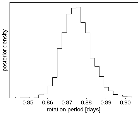
And plot the posterior distribution over rotation period:
period_samples = np.asarray(trace.posterior["period"]).flatten()
plt.hist(period_samples, 25, histtype="step", color="k", density=True)
plt.yticks([])
plt.xlabel("rotation period [days]")
_ = plt.ylabel("posterior density")
Citations#
As described in the citation tutorial, we can use citations.get_citations_for_model to construct an acknowledgement and BibTeX listing that includes the relevant citations for this model.
with model:
    txt, bib = xo.citations.get_citations_for_model()
print(txt)
This research made use of \textsf{exoplanet} \citep{exoplanet:joss,
exoplanet:zenodo} and its dependencies \citep{celerite2:foremanmackey17,
celerite2:foremanmackey18, exoplanet:arviz, exoplanet:pymc3, exoplanet:theano}.
print(bib.split("\n\n")[0] + "\n\n...")
@article{exoplanet:joss,
       author = {{Foreman-Mackey}, Daniel and {Luger}, Rodrigo and {Agol}, Eric
                and {Barclay}, Thomas and {Bouma}, Luke G. and {Brandt},
                Timothy D. and {Czekala}, Ian and {David}, Trevor J. and
                {Dong}, Jiayin and {Gilbert}, Emily A. and {Gordon}, Tyler A.
                and {Hedges}, Christina and {Hey}, Daniel R. and {Morris},
                Brett M. and {Price-Whelan}, Adrian M. and {Savel}, Arjun B.},
        title = "{exoplanet: Gradient-based probabilistic inference for
                  exoplanet data \& other astronomical time series}",
      journal = {arXiv e-prints},
         year = 2021,
        month = may,
          eid = {arXiv:2105.01994},
        pages = {arXiv:2105.01994},
archivePrefix = {arXiv},
       eprint = {2105.01994},
 primaryClass = {astro-ph.IM},
       adsurl = {https://ui.adsabs.harvard.edu/abs/2021arXiv210501994F},
      adsnote = {Provided by the SAO/NASA Astrophysics Data System}
}

...